Pooled COVID testing in the real world

[Thank you to Cathy Xue for proofreading and discussion.]

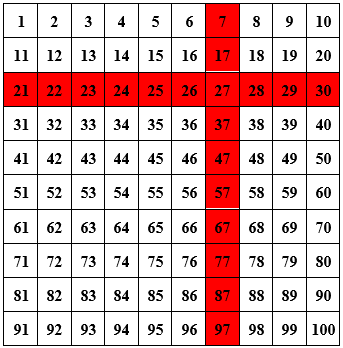
In April I wrote about pooled testing. The basic idea is that instead of testing every swab individually, labs can pool samples together in groups of 10 (say) and test each mixture (pool) for the virus. For any pool that tests positive, they can then follow up with individual tests. For example, say you’re testing 100 people, only one of whom has the virus. Testing each person individually uses up 100 tests. But if you pool the samples in groups of 10 and then re-test all the individuals in the one pool that tests positive (contains the positive sample), you only end up using 20 tests — a factor of 5 smaller than individual testing! If this doesn’t make sense, check out this great visualization.

At the time I wrote my post, there hadn’t been much discussion of pooled testing for COVID and I had just learned about the idea. My natural inclination was to ask whether the pooling scheme I just described (which I’ve since learned is called Dorfman pooling) is the most efficient one possible, or whether you can do even better by being clever. I figured out an “optimal” pooling scheme under certain constraints and assumptions and wrote about it. My analysis, however, was entirely theoretical. It was unclear whether my suggested pooling scheme would be implementable in the real world.

After reading the post, my undergraduate mentor Matt Weinberg offered to contact his friend (and former Taekwondo coach!) Alicia Zhou, who is Chief Science Officer at Color, a lab based in San Francisco. By default, many labs are prepared to do Dorfman pooling if the need for pooled testing were to arise. Our goal was to better understand how COVID testing works in practice, so as to hopefully suggest a concrete, practical pooling scheme for labs to use that would be more efficient than Dorfman. This turned into a collaborative project together with Aviad Rubinstein of Stanford, and in this post I’ll talk about some of what I learned in the process.

How COVID testing works

[Note: this section is accurate to the best of my knowledge, but might contain some inaccuracies, as much of it comes from private conversation rather than literature. Please let me know if you think I got something wrong.]

COVID testing is pretty straightforward from the consumer side; you probably know the gist. A typical experience: you go to a testing location, put a swab up your nose, and then put the swab in a liquid solution. That solution later gets tested at a lab, and eventually you get your results back. But what happens at the lab?

Samples received from a testing site are loaded onto a pipetting machine. This video should give you a sense of what these machines look like. The first step is RNA extraction. That is, before the RNA is processed, it must be separated out from everything else in the sample. This takes about 60 minutes.

The second step is molecular diagnostic: figuring out whether the virus is present. To do so, the RNA is mixed with a reagent. In general, a reagent is a chemical that reliably causes or detects a particular reaction. In the case of COVID testing, it is a chemical that reacts with genetic material from the coronavirus to produce yellow light (which can then be visually detected and quantified). But this alone is not enough: there isn’t sufficient viral RNA in the sample to produce an amount of light distinguishable from ambient noise. For this reason, the RNA first needs to be amplified, i.e. copied many times, until there’s enough of it that the amount of light reaches a certain “fluorescence threshold”. The most common method of amplification, RT-PCR, takes about 90 minutes.

RNA amplification begins by using reverse transcriptase to turn the RNA into cDNA. After that, the amplification process works in cycles. In each cycle, the cDNA is replicated, so each cycle (almost) doubles the amount of cDNA present. A sample is deemed positive if the solution reaches the fluorescence threshold (i.e. turns yellow enough) after a small-enough number of cycles. Because the reagent doesn’t perfectly target the genetic material of the virus, and because RT-PCR makes occasional errors during replication, even a sample without the virus may eventually turn yellow — it just takes much longer. Generally the amplification procedure is run for 40 cycles and a sample is deemed positive if it turns yellow by the end of that process.

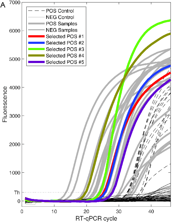
How robust is this method in terms of distinguishing positives from negatives? The answer is, quite robust. This paper by Yelin et al. discusses how many cycles it takes for a sample containing the virus and a sample not containing the virus to turn yellow. A positive sample takes about 26 cycles to turn yellow, with a standard deviation of around 6. On the other hand, almost all negative samples failed to reach the fluorescence threshold even after 45 cycles.

(Why do COVID tests have a high false negative rate, then? My understanding is that many people who are infected are swabbed before the virus has spread to their nasal cavity. In such a situation, there’s nothing to be done: the sample is indistinguishable from a true negative.)

Implications for pooling

Understanding how COVID testing works helped us understand the practical side of pooling. One of the most important takeaways for me was this: Let’s say you pool 15 negative samples and a positive sample together. Since the resulting mixture has 1/16 the concentration of virus as the original positive sample, it will take 4 more cycles for the pooled sample to reach the fluorescence threshold (since the cDNA doubles every cycle). This theoretical reasoning is verified empirically in the aforementioned Yelin et al. paper, which also examined the effect of pooling on the number of number of cycles needed to detect the virus. The lines have a slope of about 1 (at least for pools of up to 16 samples), which is what you would expect theoretically.

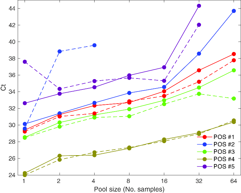
This data suggests that pools of size 16 or less shouldn’t substantially reduce sensitivity — and if the cycle threshold is pushed up to 45 or so, even testing with pools of size 64 should be fairly accurate.

Here are some other relevant facts about the testing process:

• The bottleneck for COVID testing in the United States is reagent. Swabs used to be a bottleneck, but not anymore (this is good because pooling can’t save on swabs). Machine time is also not a bottleneck. Since pooling does save on reagent, this means that pooling (and optimizing the pooling procedure) can be helpful.
• The testing process takes time on the order of hours, not days; the reason that it takes several days to get your test results backs is administrative/logistical. This means that pooling shouldn’t substantially increase the amount of time it takes to get results back.
• The pipetting machines used for testing can be programmed to pool samples in an arbitrarily complex way. This includes overlapping pools (i.e. using RNA from the same sample in multiple pools).
• However, adaptive pooling schemes are likely to be infeasible for many labs. An adaptive pooling scheme is one where you begin by pooling samples in some way, and then use the results to determine how samples are to be pooled for another round of pooling. This is likely too complicated to be implemented: all pooling should be done in parallel, at the start. However, deconvoluting the pools (i.e. following up with an individual test on any sample to determine whether it really is positive) is fine.
• While the consumer only hears a binary (positive/negative) result, internally there is an opportunity to use “number of cycles until detection” as a more precise indicator to improve test accuracy. Most simply, it likely makes sense to increase the cycle threshold for larger pools. More creatively, if a sample is in two pools, both of which just barely test negative, perhaps the sample should be tested in the deconvolution phase anyway. However, my intuition is that this wouldn’t help very much, because positives and negatives will mostly be pretty clear-cut for pools of reasonable size.

Pooling with real-world constraints

Given what we learned, we wanted to develop the optimal pooling mechanism that has the following form:

• Step 1 (pooling): Have a round of pooled testing, possibly with samples in multiple pools. Flag any samples such that all the pools they were in tested positive.
• Step 2 (deconvolution): Run individual tests on all samples flagged as potentially positive in Step 1.

There is one more constraint that I haven’t yet mentioned, because the constraint is regulatory in nature, rather than a consequence of the testing process. Specifically, the FDA’s authorization for labs to do pooled testing specifies that the labs can only include up to 5 samples in a pool — see e.g. this emergency use authorization given to LabCorp. I don’t know why the FDA decided on this limitation; my guess is that it is being overly cautious, not wanting to sacrifice any amount of test sensitivity. As we work through the math, it will become clear how the FDA’s restriction constrains us.

Let’s parametrize the problem we’re trying to optimize. First, let p be the fraction of people being tested who have the virus. p is currently around 5% nationwide, though it’s as low as 1% in New York and as high as 15% in some Southern states. When doing surveillance testing (like some colleges are currently doing), p might be as low as 0.1%. But 5% is a decent number to have in your head.

Second, let s be the number of samples we’re putting into each pool. Per the FDA regulation, s should not exceed 5.

Finally, let k be the number of pools that each sample is a part of. For example, in the Dorfman scheme (the simplest scheme, where you divide the samples up into disjoint pools, test each pool, and then follow up on the positives), k is equal to 1 because every sample is only included in one pool. In the matrix scheme (see my previous post on pooling), you put your samples into a matrix and test each row and column.

Here, k = 2 because every sample is a part of two pools (namely, the row it’s in and the column it’s in). You can also k larger than 2. For example, one way to include every scheme in three pools is to pool along every row, column, and diagonal (going down and to the right, wrapping around the square if necessary). See this (technical) footnote if you’re curious how to generalize this for arbitrary values of k.¹

So, in terms of k, s, and p, how many tests do you need to run per person you’re testing? Remember, the benchmark to beat is 1: if you test everyone individually, you use exactly one test per sample.

\begin{math} (Skip ahead to “\end{math}” if you prefer to just take my word on the formula for the number of tests needed per sample.)

For starters, every sample is in k pools, each of which has size s. This means that in Step 1 (the pooling phase), you use tests per sample. (Why? If you have n samples and each is in k pools, then that’s k*n total pools — but remember, that’s overcounting by a factor of s, because each pool is counted s times: once for every sample that’s in it.)

What about Step 2 (deconvolution)? Well, you need to test every sample such that every pool it was in tested positive. This automatically includes the p fraction of samples that are true positives: after all, if they’re true positives, then every pool they’re a part of will test positive. What about any of the 1 – p fraction of negative samples? Well, for any given pool that a negative sample is in, there’s s – 1 other samples, each of which is negative with probability 1 – p, so the probability they’re all negative is roughly , which means that the probability that the pool tests positive (contains a positive sample) is . That means that the probability that every pool that the sample is a part of tests positive² is

.

Therefore, the expected number of tests used in Step 2 per sample is

.

Combining this total with the number from Step 1, we find that all in all, this method uses

tests per person being tested.

\end{math}

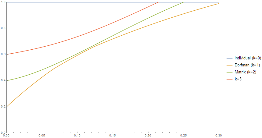
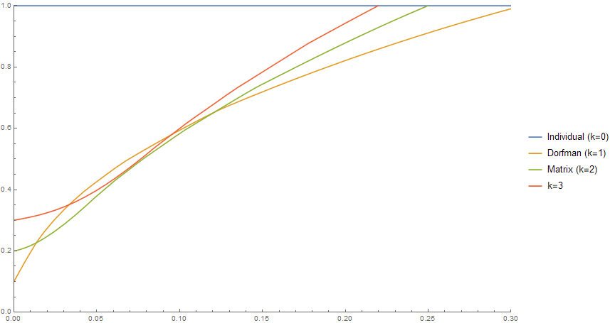
We will call the preceding quantity the efficiency of the pooling scheme (remember: lower is better, and the benchmark to beat is 1). So now that we’ve found a formula for the efficiency of a pooling scheme in terms of p, s, and k, what is the answer to our original question: what is the most efficient pooling scheme? Below is a plot that answers this question. The x-axis is the positivity rate p of the population being tested. The y-axis is the number of tests used per sample being tested (so testing everyone individually uses 1 test per sample, but lower than 1 is better). But, per the FDA regulation, we are not allowing s to be larger than 5; so the chart shows how well you can do with each method for various positivity rates, if your pools can only have up to 5 samples each.

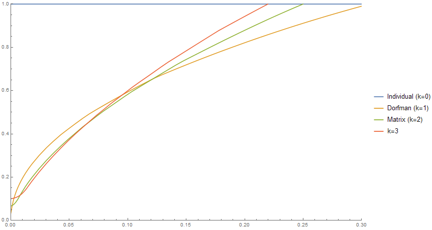
The Dorfman scheme is quite a bit better than not pooling at all: for a positivity rate of 5%, for instance, it uses 40% as many tests. And in fact, the Dorfman scheme is the best you can do — more complicated pooling schemes are less efficient! But, how much of this is just due to the limitation on our pool sizes? Well, here’s the same chart but where we allow pool sizes of up to 10 instead of 5.

The first thing to notice is that all the schemes, including Dorfman, are much more efficient for low positivity rates; for p near 0, Dorfman is twice as efficient! Additionally, the green curve (matrix pooling) now dips below the orange curve (Dorfman). This means that now we can now beat Dorfman pooling by using the matrix scheme whenever the positivity rate is between 1.4% and 12% (which is where most of the country is right now!). The biggest savings are achieved when the positivity rate is between 2% and 3%: matrix pooling saves about 15% on tests relative to the Dorfman scheme.

What if we allow ourselves to include up to 30 samples in a single pool?

Again, it’s no surprise that all the pooling schemes become much more efficient when p is small. But also, we can now do much better than Dorfman pooling when the positivity rate is on the low side. For example, if the positivity rate is 1% (as in New York, and perhaps what we might expect in surveillance testing), the k = 3 pooling scheme uses just 64% as many tests as Dorfman!

Finally, what if we remove the pool size constraint entirely and allow arbitrarily large pools? I won’t include a chart because it looks really similar to the previous one, but in some situations you can cut how many tests you need almost in half by using a more complex pooling scheme!

Why are higher values of k (i.e. each sample being included in more pools) better when the positivity rate is low? Here’s some intuition: when the positivity rate is lower, you can make the pools larger. That’s because for high positivity rates, if you make your pools large then most of the pools will test positive and then you’ll have to individually re-test most of the samples; for low positivity rates that’s less of a concern. And the good thing about large pools is that you can then afford to put each sample in more pools ( tests per sample are used in Step 1, so if s (the number of tests in a pool) is large, you can afford to make k (the number of pools each test is in) larger). Thus, lower positivity rates allow for larger pools, which in turn means you can include each sample in more pools without using too many tests in Step 1. And doing this saves you tests in Step 2, because if each sample is part of more pools, fewer negative samples will need to be re-tested in Step 2.

This intuition is supported by the huge difference in efficiency between Figure 4 (no more than 5 samples per pool) and Figure 6 (no more than 30 samples per pool) for low positivity rates. Being able to use large pools is really important for efficiency, as larger pools allow you to make full use of the power of more complex pooling schemes.

Takeaways

So, with all that said, what should the main takeaways be from this project? Here are the most important things that I’ve learned:

1. (The practical takeaway) With the limit of 5 samples per pool, you can’t beat Dorfman pooling, but Dorfman pooling is much more efficient than no pooling at all. But if this limit is relaxed, even to 10 instead of 5, it is possible to substantially improve upon the Dorfman scheme.
2. Testing regulations can be really burdensome — but sometimes you can get a lot of mileage out of relaxing them just a little. In the context of pooling, simply relaxing the cap on pool sizes from 5 to 10 not only makes the Dorfman scheme much more efficient, but also lets you save 15% on tests on top of that in some situations. Lifting the cap to 30 makes pooled testing — particularly more intricate pooling methods — even more efficient!
3. The real world is complicated, and a purely theoretical approach will often run afoul of unforeseen constraints. But if you understand the real-world aspects of your problem, theory can still be really useful — you just need to adapt your theory to real-world constraints!

^{1. Here’s one simple way to include every sample in k pools (for any k), though it has the limitation that s needs to be a prime number that is greater than or equal to k – 1. Put your samples in an s by s grid, so that every sample has an x-coordinate and a y-coordinate (between 0 and s – 1). First, pool samples according to their x-coordinates (i.e. pool the solutions to for every c). This is equivalent to pooling along the columns. Second, pool the samples along diagonals wrapping around the square (i.e. the solutions to for every c). Third, pool the samples by taking knight’s moves wrapping around the square (solutions to ), and so on. This lets you include each sample in up to s different pools. So long as s is prime, any two samples will only be together in one pool, which will be important to our math later. Finally, you can add one more set of pools by pooling along the rows.↩}

^{2. This assumes that the pools are independent. We can arrange our pools so no two overlap on more than one sample, in which case the independence assumption holds (see the previous footnote). There’s an additional question of whether we want our pools to be independent; maybe we want to put samples from one family or college dorm in the same pool. This is beyond the scope of this post, though.↩}